
Abstract
We present a machine-learning approach, based on normalizing flows, for modelling atomic solids. Our model transforms an analytically tractable base distribution into the target solid without requiring ground-truth samples for training. We report Helmholtz free energy estimates for cubic and hexagonal ice modelled as monatomic water as well as for a truncated and shifted Lennard-Jones system, and find them to be in excellent agreement with literature values and with estimates from established baseline methods. We further investigate structural properties and show that the model samples are nearly indistinguishable from the ones obtained with molecular dynamics. Our results thus demonstrate that normalizing flows can provide high-quality samples and free energy estimates without the need for multi-staging.
Export citation and abstract BibTeX RIS

Original content from this work may be used under the terms of the Creative Commons Attribution 4.0 license. Any further distribution of this work must maintain attribution to the author(s) and the title of the work, journal citation and DOI.
1. Introduction
Accurate estimation of equilibrium properties of a thermodynamic system is a central challenge of computational statistical mechanics [1, 2]. For decades, molecular dynamics (MD) and hybrid Monte Carlo [3] have been the methods of choice for sampling such systems at scale [4–6]. Recently there has been a surge in using deep learning to develop learned schemes for sampling from probability distributions in general and physical systems in particular, most notably using normalizing flows [7, 8]. Flow-based learned sampling schemes have been applied to various physical systems, from lattice field theories [9–11], to spin systems [12], to proteins [13].
Normalizing flows are appealing because of the following two properties: first, they can generate independent samples efficiently and in parallel; second, they can provide the exact probability density of their generation mechanism [14, 15]. Thus, training a flow-based model q to approximate a target distribution p (for example, the Boltzmann distribution of a physical system) yields an efficient but approximate sampler for p; re-weighting the samples by their probability density (for example, using importance sampling) can then be used to remove estimation bias [13, 16, 17]. For free energy estimation in particular, flows are interesting because they do not require samples from intermediate thermodynamic states to obtain accurate estimates, unlike traditional estimators such as thermodynamic integration [2] or the multistate Bennett acceptance ratio (MBAR) method [18]. Instead, the flow model can be used as part of a targeted estimator [11, 12, 19–24] which was demonstrated to be competitive to MBAR in terms of accuracy when applied to a small-scale solvation problem [21].
Despite their appeal for both sampling and free energy estimation of atomistic systems, constructing and training flow-based models that can rival the accuracy of already established methods remains a significant challenge. One of the reasons is that for simple re-weighting schemes such as importance sampling to be accurate in high dimensions, the model q must be a very close approximation to the target distribution p, which is hard to achieve with off-the-shelf methods. Even for common benchmark problems of identical particles, such as a Lennard-Jones system [2], successful training has thus far been demonstrated for small system sizes of up to tens of particles (for example, 38 particles in [13], 13 particles in [25]), requiring ground-truth samples from p to train in all cases. Addressing this limitation is crucial for scaling up flow-based methods to systems of interest in statistical mechanics.
In this work, we propose a flow model that is tailored to sampling from atomic solids of identical particles, and we demonstrate that it can scale to system sizes of up to 512 particles with excellent approximation quality. The model is trained to approximate the Boltzmann distribution of a chosen metastable solid by fitting against a known potential energy function. Training uses only the energy evaluated at model samples, and does not require samples from the Boltzmann distribution as ground truth. We examine the quality of the learned sampler using a range of sensitive metrics and estimate Helmholtz free energies of a truncated and shifted Lennard-Jones system (FCC phase) and of ice I (cubic and hexagonal) using a monatomic model [26]. Comparison with baseline methods shows that our flow-based estimates are highly accurate, allowing us to resolve small free energy differences.
2. Method
We begin by considering a system of N identical particles interacting via a known energy function U and attached to a heat bath at temperature T. The equilibrium distribution of this system is given by the Boltzmann distribution

where x denotes a point in the 3N-dimensional configuration space, ![$Z = \int \mathrm dx \exp[-\beta U(x)]$](https://content.cld.iop.org/journals/2632-2153/3/2/025009/revision2/mlstac6b16ieqn1.gif) is the partition function,
is the partition function,  is the inverse temperature and
  is the Boltzmann constant. Our aim is to build and train a flow model that can accurately approximate p, for atomic solids in particular.
2.1. Flow models
A flow model is a probability distribution q defined as the pushforward of an analytically tractable base distribution b through a flexible diffeomorphism f, typically parameterized by neural networks [14, 15]. Independent samples from q can be generated in parallel, by first sampling z from b and taking  . The probability density of a sample can be obtained using a change of variables,

where Jf is the Jacobian of f.
We can train q to approximate p by minimizing a loss function that quantifies the discrepancy between q and p. In this work, we use the following Kullback–Leibler divergence as the loss function

Since  is a constant with respect to the parameters of q, it can be ignored during optimization. The expectation in the final expression can be estimated using samples from b, so
  can be minimized using stochastic gradient-based methods. This loss function is appealing because it does not require samples from p or knowledge of Z, and can be optimized solely using evaluations of the energy U.
2.2. Systems and potentials
The systems considered in this work are crystalline solids consisting of N indistinguishable atoms at constant volume and temperature. The crystal is assumed to be contained in a 3-dimensional box with edge lengths  and periodic boundary conditions. A configuration x is an N-tuple
  , where
  are the coordinates of the nth atom and
 ![$x_\mathrm{ni} \in [0, L_i/\sigma]$](https://content.cld.iop.org/journals/2632-2153/3/2/025009/revision2/mlstac6b16ieqn10.gif) with σ being a characteristic length scale of the system (here the particle diameter). By expressing x in reduced units, Z and all probability densities become dimensionless.
with σ being a characteristic length scale of the system (here the particle diameter). By expressing x in reduced units, Z and all probability densities become dimensionless.
The potentials used in this work are invariant to global translations (with respect to periodic boundary conditions) and arbitrary atom permutations. Both of these symmetries are incorporated into the model architecture; that is, we design the base distribution b and the diffeomorphism f such that the density function q is invariant to translations and atom permutations, as well as compatible with periodic boundary conditions. We explain how this is achieved in the following paragraphs.
2.3. Model architecture
Our base distribution b is constructed as a lattice with N sites that have been randomly perturbed and permuted as illustrated in figure 1. Starting from a lattice  , a configuration
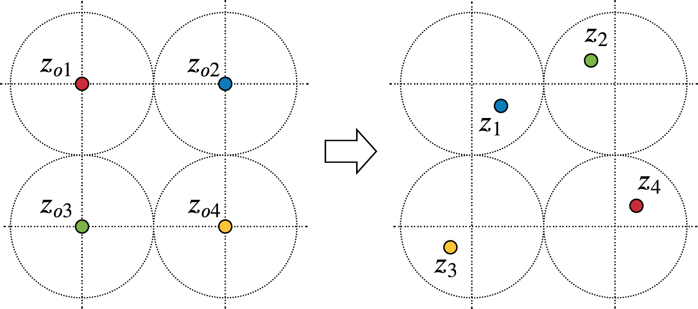
  is generated by independently adding spherically-truncated Gaussian noise to each lattice site, followed by a random permutation of all atoms. The truncation is chosen such that no two neighbouring atoms can swap lattice sites, so that after the permutation, all atoms can be traced back to the site they originated from. This construction yields a base distribution that can be trivially sampled from, and has a permutation-invariant probability density function that can be evaluated exactly.

Figure 1. Illustration of generating samples from the base distribution in 2D: atoms arranged on a lattice (left) are perturbed with truncated Gaussian noise and randomly permuted (right).
Download figure:
Standard image High-resolution imageOur diffeomorphism f is implemented as a sequence of K invertible functions composed such that  . Each function fk
is parameterized by a separate neural network, whose parameters are optimized by the loss in equation (3). We implement the functions fk
using an improved version of the model proposed in [21]. In this model, each fk
transforms element-wise either one or two coordinates of all atoms as a function of all remaining coordinates. The transformation of each coordinate is implemented using circular rational-quadratic splines [27], which ensures that the transformation is nonlinear, invertible and obeys periodic boundary conditions. The spline parameters are computed as a function of the remaining coordinates using multiple layers of self-attention, a neural-network module commonly used in language modelling [28]. Wirnsberger et al [21] showed that a diffeomorphism f parameterized this way is equivariant to atom permutations, which means that permuting the input of f has the same effect as permuting the output of f. As also shown by [25, 29], the combination of a permutation-invariant base distribution with a permutation-equivariant diffeomorphism yields a permutation-invariant distribution q, as desired. More implementation details are provided in the supplementary material (available online at stacks.iop.org/MLST/3/025009/mmedia).
. Each function fk
is parameterized by a separate neural network, whose parameters are optimized by the loss in equation (3). We implement the functions fk
using an improved version of the model proposed in [21]. In this model, each fk
transforms element-wise either one or two coordinates of all atoms as a function of all remaining coordinates. The transformation of each coordinate is implemented using circular rational-quadratic splines [27], which ensures that the transformation is nonlinear, invertible and obeys periodic boundary conditions. The spline parameters are computed as a function of the remaining coordinates using multiple layers of self-attention, a neural-network module commonly used in language modelling [28]. Wirnsberger et al [21] showed that a diffeomorphism f parameterized this way is equivariant to atom permutations, which means that permuting the input of f has the same effect as permuting the output of f. As also shown by [25, 29], the combination of a permutation-invariant base distribution with a permutation-equivariant diffeomorphism yields a permutation-invariant distribution q, as desired. More implementation details are provided in the supplementary material (available online at stacks.iop.org/MLST/3/025009/mmedia).
Finally, we incorporate the translational symmetry into the above architecture as follows. We fix the coordinates of an arbitrary reference atom (say x1), and use the flow model to generate the remaining N − 1 atom coordinates as described above. Then, we globally translate the atoms uniformly at random (under periodic boundary conditions), so that the reference atom can end up anywhere in the box with equal probability. Since the index of the reference atom and its original position are known and fixed, we can reverse this operation in order to obtain the probability density of an arbitrary configuration. This procedure yields a translation invariant probability density function that can be calculated exactly.
A key feature of our model architecture is that we can target specific crystal structures by encoding them into the base distribution. For example, if we are interested in modelling the hexagonal phase of a crystal, we can choose the lattice of the base distribution to be hexagonal. Empirically, we find that, after training, the flow model becomes a sampler for the (metastable) crystal state that we encode in the base distribution, and does not sample configurations from other states. Thus, by choosing the base lattice accordingly, we can guide the model towards the state of interest, without changing the energy function or using ground-truth samples for guidance.
3. Results
We train the models on two different systems. The first is a truncated and shifted Lennard-Jones (LJ) crystal in the FCC phase at reduced temperature and density values of 2 and 1.28, respectively, employing a reduced cutoff of 2.7 as in [30]. The second is ice I modelled as monatomic Water (mW) [26] in the diamond cubic (Ic) and hexagonal (Ih) phases at a temperature of 200 K and a density of approximately  similar to [31]. All further simulation details are provided in the supplementary material.
Code for reproducing the experiments and pre-trained models are provided at https://github.com/deepmind/flows_for_atomic_solids. The code uses JAX [32], Haiku [33] and Distrax [34] for building and training models.
3.1. Evaluation of model samples
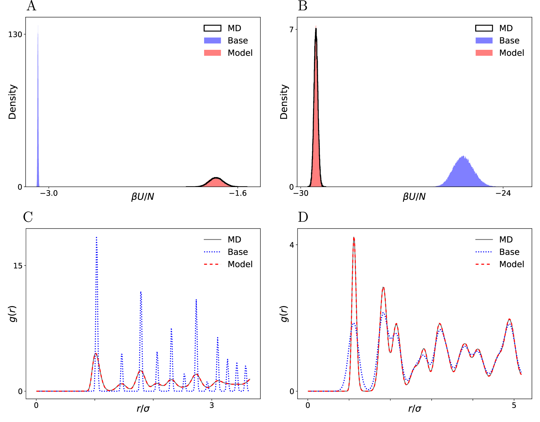
To assess the quality of our trained models, we compare against MD. We ran NVT simulations of the target systems using the simulation package LAMMPS [35]. Figure 2 shows the energy histogram and radial distribution function (RDF) of the Lennard-Jones FCC crystal and of cubic ice, as computed by samples from the base distribution, the trained model, and MD. The RDF g(r) is the ratio of the average number density at a distance r of an arbitrary reference atom and the average number density in an ideal gas at the same overall density [2]. By construction, the base distribution captures the locations of the peaks in the RDF correctly, but its energy histogram is far off compared to the MD result. The energy histograms and the RDFs computed from model samples, however, are nearly indistinguishable from MD in both systems. Importantly, no unbiasing or re-weighing was necessary to obtain this quality of agreement. The results for hexagonal ice show a similar level of agreement (see supplementary material). These results demonstrate that the mapping f successfully transforms the base distribution into an accurate sampler.

Figure 2. Energy histograms (A) and (B) and radial distribution functions (C) and (D) of the base distribution, the fully trained model and MD simulation data, for the 500-particle LJ system (left) and the 512-particle cubic ice system (right).
Download figure:
Standard image High-resolution imageTo demonstrate that the trained model becomes a sampler of the (metastable) crystal structure that we have encoded into the base distribution, we computed histograms of the averaged local bond-order parameter q6 [36] that was designed to discriminate between different phases (see figure 3). We can see that the two histograms are well separated and agree with MD, showing that the model does indeed become an accurate sampler of only the crystal state encoded in the base distribution. If that were not the case, we could have enforced it by adding a biasing potential to the energy, as commonly done in nucleation studies that employ umbrella sampling [37].

Figure 3. Histograms of averaged local bond order parameter q6 for 512-particle cubic and hexagonal ice. Solid lines indicate the histograms from MD samples; shaded areas from model samples. The vertical lines mark the maximum and minimum values seen in 1 M bond order parameters for each of the two model histograms.
Download figure:
Standard image High-resolution image3.2. Free energy estimation
Next, we use the trained flow models to estimate the Helmholtz free energy F for various system sizes, which is given by [2]

We note that the thermal de Broglie wavelength does not appear in the above expression as we set it to σ, following [38], and absorb it into Z by expressing x in reduced units. We then estimate  by first defining a generalized work function [19]

The average work value  is also our training objective in equation (3). We then harness the trained flow to draw a set of samples
  from q and estimate
  via the targeted free energy perturbation estimator [19]

The above estimation method, referred to as learned free energy perturbation (LFEP) in combination with a learned model [21], is appealing, because it does not require samples from p for either training the model or for evaluating the estimator.
Although the approximation in equation (6) becomes exact in the limit of an infinite sample size, to obtain accurate results for a finite sample set we require sufficient agreement between the proposal and the target distributions [19, 21]. Since  quantifies the pointwise difference between
  and
and  (up to an additive constant), the distribution of generalized work values is a good metric for assessing the quality of the flow for free energy estimation.
Figure 4 compares distributions of work values computed for the base distribution and for the fully trained model. From the non-negativity of the Kullback–Leibler divergence in equation (3) it follows that  , with equality if and only if q and p are equal. Therefore, the gap between the average work value and
  (which we aim to estimate) quantifies how accurately the model q approximates the Boltzmann distribution p; for a perfect model, we would expect to see a delta distribution located at
  [19]. The work values obtained with the trained model are indeed sharply peaked near our MBAR estimate of
  . On a qualitative level, this shows a clear benefit of LFEP [21] over the original FEP estimator corresponding to f being the identity map, which failed to converge on this problem.

Figure 4. Histograms of work values ( ) per particle from base and model samples for 500-particle LJ crystal (A) and 512-particle cubic ice (B). The dashed vertical line marks
  as estimated by MBAR (enlarged in inset). Upper insets: scatter plots of model density vs approximately normalized target density
  computed from model samples, where the model is either the base distribution or the fully trained model and
  is the MBAR estimate. The dotted diagonal marks the identity.
Download figure:
Standard image High-resolution image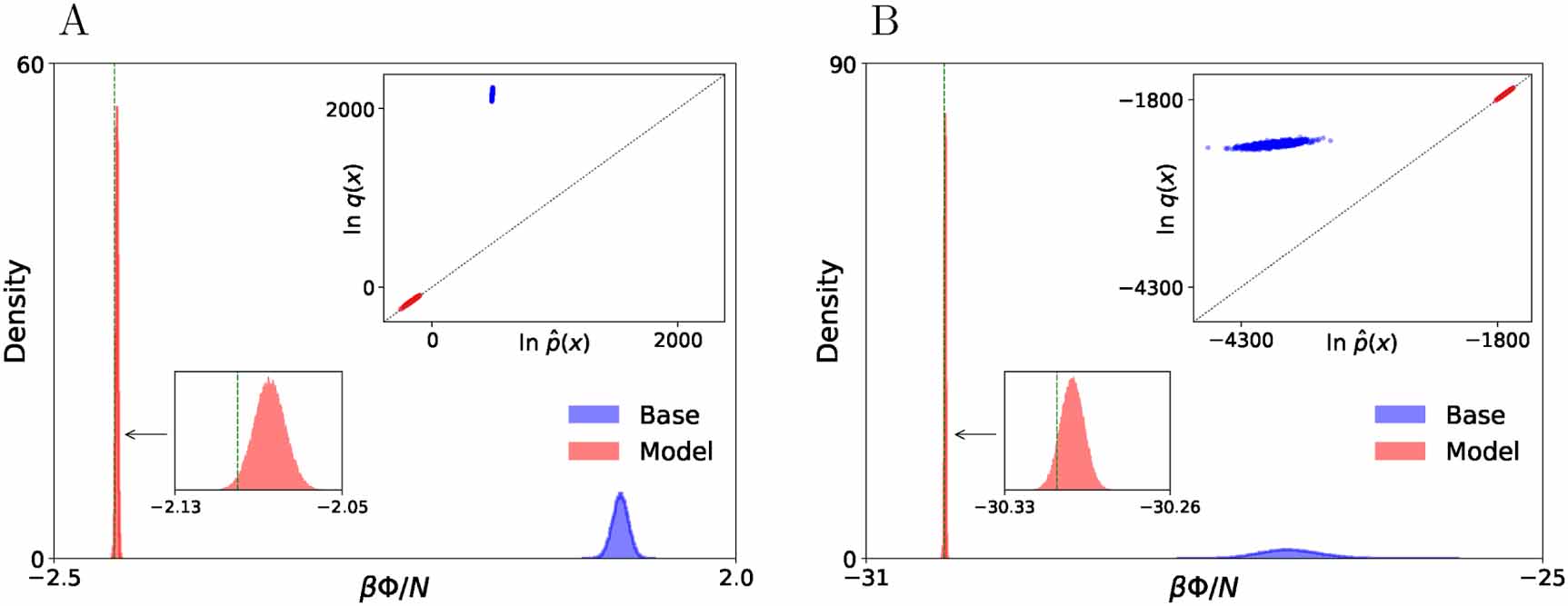
Using the same trained model as in LFEP, we can also employ a learned version of the bidirectional BAR estimator (LBAR) [21, 39]. LBAR uses samples from both the base distribution b and from the target p and is known to be the minimum variance estimator for any asymptotically unbiased method [40]. The downside compared to LFEP is that an additional MD simulation needs to be performed to obtain samples from p for computing the estimator (but not for training the model).
To verify the correctness of the flow-based free energy estimates, we require an accurate baseline method. The Einstein crystal (and molecule) method [38, 41] and lattice-switch Monte Carlo (LSMC) [42] are common choices for computing solid free energies with different trade-offs. While the former is conceptually simple, we found it challenging to optimize it to high precision, which is consistent with previously reported results [30, 38]. The latter is known to be accurate but provides only free energy differences between two compatible lattices rather than absolute free energies. We therefore tested MBAR as an alternative estimator on this problem and found it yields sufficiently accurate absolute free energy estimates to serve as a reference.
A quantitative comparison of free energy estimates for both systems and different system sizes is shown in table 1 (see also supplementary material). For LFEP we use S samples from the base distribution b; for LBAR we use S samples from b, plus another S samples from the target p obtained by MD; for MBAR we use a sufficiently large number of intermediate states between b and p to obtain good accuracy, which we sample using MD (see caption of table 1 for exact numbers). Overall, we find excellent agreement of the learned estimators with MBAR for both LJ and ice. The LBAR estimates exhibit lower statistical uncertainties than LFEP across the board, with error bars on the order of  per particle. We find it remarkable, however, that LFEP can yield comparable accuracy in most cases without access to MD samples for training or estimation, and without the need for defining intermediate states. Finally, we compute the Helmholtz free energy difference between cubic and hexagonal ice for 216 particles by subtracting the two LFEP estimates in table 1. This yields a value of
  which is in good agreement with the reported Gibbs free energy difference of
  obtained with LSMC simulations at atmospheric pressure [31].
Table 1. Helmholtz free energy estimates,  , obtained with 2 M,
  M and
M and  k samples for LFEP, LBAR and MBAR for LJ, and 2 M,
  M and
M and  k samples for ice. Parentheses show the uncertainties in the last digits (two standard errors); error bars for LFEP and LBAR were computed using ten independently trained models, so they quantify uncertainty both due to randomness in training and due to finite sample size in estimation; error bars for MBAR were computed across ten independent estimates. The literature value for LJ is 3.11(4) for 256 particles [30]; the literature value for mW is unknown. See supplementary material for further details.
| System | N | LFEP | LBAR | MBAR |
|---|---|---|---|---|
| LJ | 256 | 3.10800(28) | 3.10797(1) | 3.10798(9) |
| LJ | 500 | 3.12300(41) | 3.12264(2) | 3.12262(10) |
| Ice Ic | 64 | −25.16311(3) | −25.16312(1) | −25.16306(20) |
| Ice Ic | 216 | −25.08234(7) | −25.08238(1) | −25.08234(5) |
| Ice Ic | 512 | −25.06163(35) | −25.06161(1) | −25.06156(3) |
| Ice Ih | 64 | −25.18671(3) | −25.18672(2) | −25.18687(26) |
| Ice Ih | 216 | −25.08980(3) | −25.08979(1) | −25.08975(14) |
| Ice Ih | 512 | −25.06478(9) | −25.06479(1) | −25.06480(4) |
4. Discussion
In summary, we have proposed a normalizing-flow model for solids consisting of identical particles and have demonstrated that it can be optimized to approximate Boltzmann distributions accurately for system sizes of up to 512 particles, without requiring samples from the target for training. We have shown that flow-based estimates of RDFs, bond-order parameters and energy histograms agree well with MD results, without the need for an unbiasing step. A detailed comparison of free energy estimates further verifies that our flow-based estimates are correct and accurate. Our work therefore clearly demonstrates that flow models can approximate single states of interest with high accuracy without training data, providing a solid foundation for follow-up work.
A current limitation of our proposed method is the computational cost of training. Although generating samples from the model and obtaining their probability density is efficient as it is trivially parallelizable, training the model with gradient-based methods is inherently sequential. While training took only a day on the smallest system (64-particle mW), reaching convergence of the free energy estimates for the biggest systems (512-particle mW and 500-particle LJ) took approximately 3 weeks on 16 A100 GPUs (details in the supplementary material). Therefore, our approach is best suited for applications where the cost of training can be amortized across several evaluations. In particular, a promising research direction is training a single model parameterized by state variables or order parameters (such as temperature, pressure, particle density, etc), so that a range of states or systems can be approximated at the cost of training only once.
With rapid improvements in model architectures, optimizers and training schemes, it seems likely that this type of approach can be scaled up to larger system sizes and other types of challenging systems, such as explicit water models with electrostatic interactions and rotational degrees of freedom, in the future. The application and adaptation of increasingly suitable normalizing flows is a very active area of research, for example, the concurrent work on solids in [43], yielding increasingly flexible flows for progressively more general systems. The end-to-end differentiability of our approach (or one more general) could be leveraged to address difficult inverse material design problems, extending recent MD-based approaches [44].
Data availability statement
The data that support the findings of this study are openly available at the following URL/DOI: https://github.com/deepmind/flows_for_atomic_solids.
Acknowledgments
We would like to thank our colleagues Stuart Abercrombie, Danilo Jimenez Rezende, Théophane Weber, Daan Wierstra, Arnaud Doucet, Peter Battaglia, James Kirkpatrick, John Jumper, Alex Goldin and Guy Scully for their help and for stimulating discussions.